LU decomposition in TI-84

As an extension to a previous entry on doing LU decomposition in Nspire and R, the TI-84 is covered here. There is no built-in function like in the Nspire for this, but there are many programs available online, with most of them employing a simple Doolittle algorithm without pivoting.

The non-pivoting program described here for the TI-84 series is with a twist. No separate L and U matrix variables are used and the calculations are done in place with the original input matrix A. The end result of both L and U are also stored in this input matrix. This is made possible by the property of the L and U matrices in this decomposition are triangular. Therefore, at the little price of some mental interpretation of the program output, this program will take up less memory and run a little faster than most simple LU decomposition programs online for the same class of calculator. From a simple benchmark with a 5 x 5 matrix, this program took 2 seconds while another standard program took 2.7 seconds.

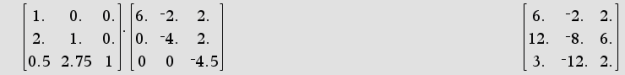
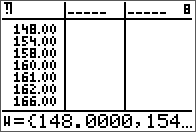
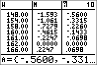
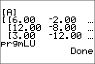
The input matrix A.

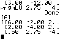
Results are stored in the same matrix.

L, U, and verification.

Shipping option decision by linear regression on TI-84

An online store offered the following shipping options:

Monday – $142
Tuesday – $86
Friday – $63

Applying linear regression in TI-84, the following parameters are obtained.

Plotting the results in Stat Plot:

It therefore appears delivery on Tuesday is the most appealing choice.

Durbin-Watson statistic in TI-84

Unlike the more sophisticated TI-89 and Nspire, the Durbin-Watson statistic is not included in the TI-84. Yet, calculating it is fairly straight-forward using list functions.

This statistics of regression is given as

where e is the residual list of values. To obtain this list (using a previous multiple regression example), simply subtract the actual values from the regression formula (Y7 below):

 

Finally, run the formula below for answer.

Coefficient of determination for Multiple linear regression in TI-84 Plus

After determining the parameters of multiple linear regression in TI-84 (which do not have any direct built-in function support of this calculation), the coefficient of determination can also be easily calculated using the rich set of list functions supported by TI-84. Following the previous example, the dependent variable is in Sales list, the other two independent variables are Size and Dist lists.

The Yhat list is to be prepared first. This lists store the predicted values using the regression parameters determined in the previous installment.

Next, the mean of Y and Yhat are calculated and stored to a handy list S.

Furthermore, three lists SYY, SYhYh, SYYh are calculated respectively.

The result is obtained by the formula below.

Graphical visualization of data distribution in TI-84 and R

For visualizing data distribution, the TI-84 Stat plot can provide some insights. Using the same data set as in the previous installment on Shapiro-Wilk test, TI-84 Stat plot is a quick and convenient tool.

 

In R, the command qqnorm() will show the following plot for the same data.

P value of Shapiro-Wilk test on TI-84

In previous installment, the Shapiro-Wilk test is performed step by step on the TI-84.

To calculate the p-value from this W statistic obtained, the following steps can also be done on the TI-84 using some standard statistics function. Note that the approximation below are for the case 4 ≤ n ≤ 11.

The mean and standard deviation are derived using the below equations.

The W statistic is assigned from the correlation calculation results, and another variable V is calculated for the transformed W.

Finally, the standardized Z statistic and p-value is calculated using the mean, standard deviation, and the transformed W value.
 

Performing Shapiro-Wilk test on TI-84

On TI-84, although the Shapiro-Wilk test is not available as built-in function, it is possible to calculate the W statistics by using the calculator’s rich set of list and statistics function. It is not trivial, but doable.

First set up a list of sample values. Using the example from the original Shapiro-Wilk paper, the samples are input into a list called W, while the N variable denotes the dimension and U stores inverse of its square root. The data sample in W must be sorted in ascending order.

 

Next is to generate the M list based on W. This list is to calculate the inverse normal distribution based on the index value and the dimension of W list. Doing this in TI-84 is easy with the help of the seq() function. The complete expression is:
seq(invNorm( (I-0.375) / (N+0.25), 0, 1), I, 1, N, 1)

 

Now that the List M is ready, it is time to derive the sum of square of it and we store it into variable m (not the list M).

Since the approximation algorithm is used instead of look up table as proposed in the original paper, the next step is to prepare List A. This list is arranged in such a way that the first two and last two elements have different calculation than all the others. The last two values (N-1, N) of List A are prepared in the Y5 and Y6 equations. These are approximating equations. The first two elements are the negation of these two in a particular order.
 

One more variable, ε, has to be calculated at this point before we generate List A.
(m - 2*M(N)² - 2*M(N-1)²) / (1 - 2*Y6² - 2*Y5²)

Next is to generate the List A. As explained, four elements namely the first, second, N-1, and N elements of this list is calculated unlike all other elements. The screen below is for all except that four special elements.

The remaining steps for the four elements of this List A are then carried out as below.

Finally, all three lists are ready for calculation.

To calculate the W statistics, use the Linear Regression function in the TI-84 as below for W and A. The correlation coefficient r² is the W statistics as shown in R. See the next installment for the Z statistic and P value calculations from this W statistic, also on the TI-84.

 

Micro SD card performance with different adaptor

There are several way to connect a micro SD card to a PC. The most popular being a versatile USB card reader that is capable to read different storage media. There are also built-in card reader on notebook computer.

Since the Android phone supported USB external media via OTG interface, there is a new kind of micro SD adapter on the market that work with both mobile device and PC, and are made very compact like the one on the right below.

To compare whether there will be difference in access speed, a simple test is performed using CrystalDiskMark with the two adapter devices above. Three groups of 10 sample read data (an internal SD reader of a notebook computer, a standard USB interface, and a USB 3.0 interface) are collected for the same micro-SD card which is a SanDisk 32GB class 4. The data are analysed using the ANOVA function available on the TI-84.

Looking at the p-value, there is a significant difference between any of the mean reading speed.

Moving average calculation on scientific vs financial calculator

The idea behind moving average is very simple. It used to be quite cumbersome for older generations of calculator to do this sort of calculation. With modern models, this is a piece of cake as the List feature is almost becoming a standard feature.

For the popular TI-84 series, the list feature can be used to store values into variables. Not only can the list be named, the name assigned can also consist of multiple characters. With the list defined, the moving averages can easily be calculated with arbitrary parameters.

On the financial model arena, the HP17bII+ is a special breed alongside its popular and successful line of signature financial calculator HP12c. The manual for the 17b provided an example that make use of the built-in solver for this. The menu driven 17b is quite convenient to use.

Date arithmetic in TI Nspire

The TI Nspire CX (and also 83, 84, 89 series) provided a useful date function, dbd(), for finding the number of days between two input dates. However, after nothing turn up searching for function to perform days addition, a quick and dirty program is developed by taking advantage of this built-in function.

The program takes two parameters: a date and the number of day to add, and basically brute force a range of dates to check if the dbd() function returns a value equals that of the intended number of days to add. The program assumed the format DDMM.YY, while the built-in dbd() function accepts format in either DDMM.YY or MM.DDYY.