Approximating the value of Pi by Monte Carlo method in Nspire and NVIDIA GPU

The value of pi can be approximated by Monte Carlo method. This can easily be done with any thing from a programmable calculator like the Nspire, or much more efficiently in parallel computing devices like GPU.

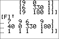
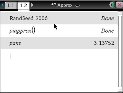
Writing code in the Nspire is straight forward. Nspire Basic provided random number functions like RandSeed(), Rand(), RandBin(), RandNorm() etc.

To implement the Monte Carlo method in GPU, random numbers are not generated in the CUDA kernel functions, but in the main program using CuRand host APIs. On the NVIDIA GPU, CuRand is an API for random number generation, with 9 different types of random number generators available. At first I picked one from the Mersenne Twister family (CURAND_RNG_PSEUDO_MT19937) as the generator but unfortunately this returned a segmentation fault. Tracing the call to curandCreateGenerator revealed the status value returned is 204 which means CURAND_STATUS_ARCH_MISMATCH. It turns out this particular generator is supported only on Host API and architecture sm_35 or above. Eventually settled with CURAND_RNG_PSEUDO_MTGP32. The performance of this RNG is closely tied to the thread and block count, and the most efficient use is to generate a multiple of 16384 samples (64 blocks × 256 threads).

On a side note, to use the CuRand APIs in Visual Studio, the CuRand library must be added to the project dependencies manually. Otherwise there will be error in the linking stage since the CuRand is dynamically linked.

On the Nspire, using 100,000 samples, it took an overclocked CX CAS 790 seconds to complete the simulation. The same Nspire program finishes in 8 seconds in the PC version running on a Core i5.

On the GPU side, CUDA on a GeForce 610M finished in a blink of an eye for the same number of iterations.

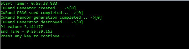
To get a better measurement on the performance, the number of iteration is increased to 10,000,000 and the result on performance is compared to a separately coded Monte Carlo program for the same purpose that run serially instead of parallel CUDA. The GPU version took 296 ms, while the plain vanilla C ran for 1014 ms.

Multiple linear regression in TI-84 Plus

Advanced feature like multiple linear regression is not included in the TI-84 Plus SE. However, obtaining the regression parameters need nothing more than some built-in matrix operations, and the steps are also very easy. For a simple example, consider two independent x variables x₁ and x₂ for a multiple regression analysis.

Firstly, the values are input into lists and later turned into matrices. L1 and L2 are x₁ and x₂, and L3 is the dependent variable.

Convert the lists into matrices using the List>matr() function. L1 thru L3 are converted to Matrix C thru E.

Create an matrix with all 1s with the dimension same as L1 / L2. And then use the augment() function to create a matrix such that the first row is L1 (Matrix C), second row is L2 (Matrix D), and the third row is the all 1s matrix. In this example we will store the result to matrix F. Notice that since augment() takes only two argument at one time, we have to chain the function.

The result of F and its transform look like below.

Finally, the following formula is used to obtain the parameters for the multiple regression

([F]t * [F])-1 * [F]t * [E]

The parameters are expressed in the result matrix and therefore the multiple regression equation is

y = 41.51x1 - 0.34x2 + 65.32

See also this installment to determine the correlation of determination in a multiple linear regression settings also using the TI-84.

TI-84 Plus Pocket SE and the Simplex Algorithm

The TI-84+ Pocket SE is the little brother of the TI-84 Plus. They are almost identical in terms of screen resolution, processor architecture and speed, and also the OS. The Pocket version measured only 160 x 80 x 21mm in dimension and weighted at 142g, considerably more compact than the classic version.

This little critter is full of features from the 2.55 MP OS. It will easily blow away the mainstream Casio series of the same size like the fx991 and even fx5800P with TI’s built-in advanced functions like ANOVA. Nevertheless, the TI-84 Plus series is still considered a stripped down version of the TI Nspire and TI-89 Titanium, and as such personally I do not expect or intent to run on it sophisticated calculations or programs like the Nelder-Mead algorithm that fits comfortably on the Nspire or Titanium.

Having said that, many complex calculation can easily be accomplished with the rich set of advanced features available out-of-the box in the TI-84, even without programming. One such example is the linear programming method implemented in the simplex algorithm for optimization. Consider the following example: In order to maximize profit, number of products to be produced given a set of constraints can be determined by linear programming. This set of constraints can be expressed in linear programming as system of equations as

8x + 7y ≤ 4400   :Raw Material P
2x + 7y ≤ 3200   :Raw Material Q
3x + y ≤ 1400    :Raw Material R
x,y ≥ 0

In the above, two products are considered by variable x and y, representing the constraints for product A and B respectively. Each of the first three equations denote the raw material requirements to manufacture each product, for material P, Q, and R. Specifically, product A requires 8 units of raw material P, 2 units of raw material Q, and 3 units of raw material R. The total available units for these three raw materials in a production run are 4400, 3200, and 1400 units respectively. When using the Simple Algorithm to maximize the function

P = 16x + 20y

which represents the profits for product A and B are $16 and $20 each, the tableau below is set up initially with slack variables set as

  8   7 1 0 0 0 4400
  2   7 0 1 0 0 3300
  3   1 0 0 1 0 1400
-16 -20 0 0 0 1    0

Using the *row() and *row+() matrix function, the Simplex Algorithm can be implemented without even one line of code. The final answer is obtained as 11200 which is the maximum profit by producing 200 Product A and 400 Product B.