Category Archives: Nvidia

Visualizing a MLP Neural Network with TensorBoard

The Multi-Layer Perceptron model is supported in Keras as a form of Sequential model container as MLP in its predefined layer type. For visualization of the training results, TensorBoard is handy with only a few line of code to add to the Python program.

log_dir="logs/fit/" + datetime.datetime.now().strftime("%Y%m%d-%H%M%S")
tensorboard_callback = tf.keras.callbacks.TensorBoard(log_dir=log_dir, histogram_freq=1)

Finally add callbacks to the corresponding fitting model command to collect model information.

history = model.fit(X_train, Y_train, validation_split=0.2,
epochs=100, batch_size=10
,callbacks=[tensorboard_callback])

tfb1

Once the training is completed, start the TensorBoard and point browser to the designated port number.

Click on the Graph tab to see a detailed visualization of the model.
tfb2

Click on the Distributions tab to check the layer output.
tfb3

Click on the Histograms tab for a 3D visualization of the dense layers.
tfb4


Profiling machine learning applications in TensorFlow

TensorFlow provided package timeline by using the import from tensorflow.python.client

from tensorflow.python.client import timeline

This is useful for performance profiling TensorFlow application with graphical visualization similar to the graphs generated from the CUDA Visual Profiler. With a little tweak in the machine learning code, TensorFlow applications can store and report performance metrics of the learning process.
tfprofile3

The design of the timeline package made it easy to add profiling by simply adding code below.

run_options = tf.RunOptions(trace_level=tf.RunOptions.FULL_TRACE)
run_metadata = tf.RunMetadata() 

It is also required to instruct the model to compile with the profiling options:

model.compile(optimizer='adam',
loss='sparse_categorical_crossentropy',
metrics=['accuracy'],
options=run_options,
run_metadata=run_metadata)

With the sample mnist digits classifier for TensorFlow, the output shown Keras history are saved and can be later retrieved to generate reports.
tfprofile2

Finally, using the Chrome tracing page ( chrome://tracing/ ), the performance metrics persisted on file system can be opened for verification.
tfprofile1


TensorFlow and Keras on RTX2060 for pattern recognition

The MNIST database is a catalog of handwritten digits for image processing. With TensorFlow and Keras training a neural network classifier using the Nvidia RTX206 GPU is a walk in the park.
mnist2

Using the default import of the MNIST dataset using tf.keras, which comprises of 60,000 handwritten digits images in 28 x 28 pixels, the training of a neural network to learn classifying it could be accomplished in a matter of seconds, depending on the accuracy. The same learning done on ordinary CPU is not as quick as GPU for architectural differences. In this sample run, the digit “eight” is correctly identified using the neural network.
mnist4.PNG

A simple comparison of the training result of the MNIST database on my RTX2060 with varying training samples depicts slight differences in the final accuracy.
mnist1


More test driving of Tensorflow with Nvidia RTX 2060

By following the TensorFlow guide, it is easy to see how TensorFlow harnesses the power of my new Nvidia RTX 2060.

The first one is image recognition. Similar to the technology used in a previous installment on neural network training with traffic images from CCTV captured, a sample data set of images with classification of fashion objects are learnt by using TensorFlow. In that previous installment, Amazon Web Service cloud with a K520 GPU instance is used for the model training. In this blog post, the training is actually taking place in the Nvidia RTX 2060.

tfimg1

Another classic sample is the regression analysis, from the Auto MPG data set. With a few line of code, TensorFlow clean up the data set to remove unsuitable values and convert categorical values to numeric ones for the model.

tfimg2

Test driving Nvidia RTX 2060 with TensorFlow and VS2017

Finally my new laptop that sports the new GeForce Nvidia RTX 2060 arrived. It is time to check out the muscle of this little beast with the toolset I’m familiar with.

On the hardware, the laptop is a i7-8750 and 16G RAM with a Turing architecture based GeForce RTX 2060.

rtx1.PNG

The laptop came with full drivers installed. Nevertheless I downloaded the latest drivers and CUDA for the most up-to-date experience. The software include Nvidia GeForce drivers, Visual Studio Express 2017, CUDA Toolkit, and TensorFlow.

rtx6.PNG

Be careful when trying all these bleeding edge technologies, not only because TensorFlow 2.0 is currently in Alpha, compatibility issues may haunt like with previous 1.x TensorFlow on CUDA 10.1. I have to fallback to 10.0 to have TF happy with it (although one can always choose the compile from source approach).

rtx2

And here are my favorite nbody and Mandelbrot simulation, and also the Black Scholes sample in CUDA. The diagnostic tool in VS gives a nice real time profiling interface with graphs.

rtx5

Finally for this test drive – TensorFlow with GPU. The installation is smooth until I tried to verify TF on GPU. After several failed attempts I realized it could be that CUDA 10.1 may not be compatible with the TF version installed. There are couples of suggested solutions out there, including downgrading to CUDA 9, but since my GPU is the Turing series this is not an option. Actually TF supports CUDA 10 since v.13. So I finally decided to fall back CUDA to 10.0 from 10.1 and it worked!rtx7


Logistic Regression – from Nspire to R to Theano

Logistic regression is a very powerful tool for classification and prediction. It works very well with linearly separable problem. This installment will attempt to recap on its practical implementation, from traditional perspective by maximum likelihood, to more machine learning approach by neural network, as well as from handheld calculator to GPU cores.

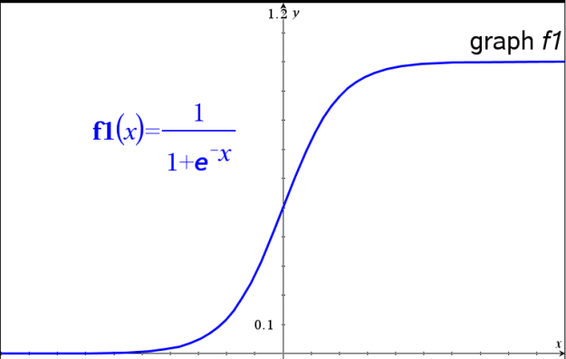
The heart of the logistic regression model is the logistic function. It takes in any real value and return value in the range from 0 to 1. This is ideal for binary classifier system. The following is a graph of this function.
theanologistic1

TI Nspire

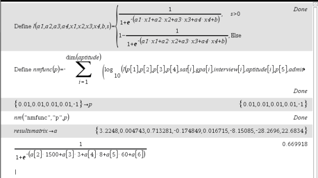
In the TI Nspire calculator, logistic regression is provided as a built-in function but is limited to single variable. For multi-valued problems, custom programming is required to apply optimization techniques to determine the coefficients of the regression model. One such application as shown below is the Nelder-Mead method in TI Nspire calculator.

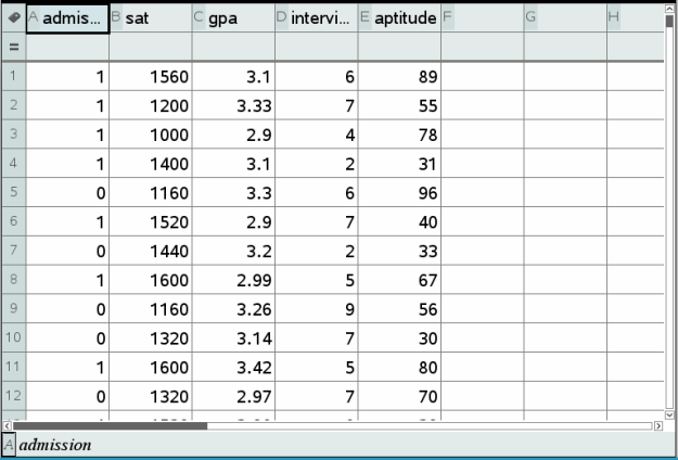
Suppose in a data set from university admission records, there are four attributes (independent variables: SAT score, GPA, Interview score, Aptitude score) and one outcome (“Admission“) as the dependent variable.
theano-new1

Through the use of a Nelder-Mead program, the logistic function is first defined as l. It takes all regression coefficients (a1, a2, a3, a4, b), dependent variable (s), independent variables (x1, x2, x3, x4), and then simply return the logistic probability. Next, the function to optimize in the Nelder-Mead program is defined as nmfunc. This is the likelihood function on the logistic function. Since Nelder-Mead is a minimization algorithm the negative of this function is taken. On completion of the program run, the regression coefficients in the result matrix are available for prediction, as in the following case of a sample data with [GPA=1500, SAT=3, Interview=8, Aptitude=60].

theanologistic2(nspire1)

R

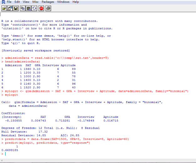
In R, as a sophisticated statistical package, the calculation is much simpler. Consider the sample case above, it is just a few lines of commands to invoke its built-in logistic model.
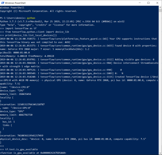
theano-new2

Theano

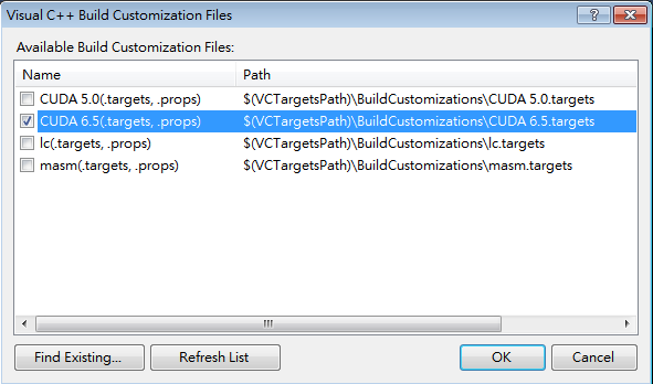
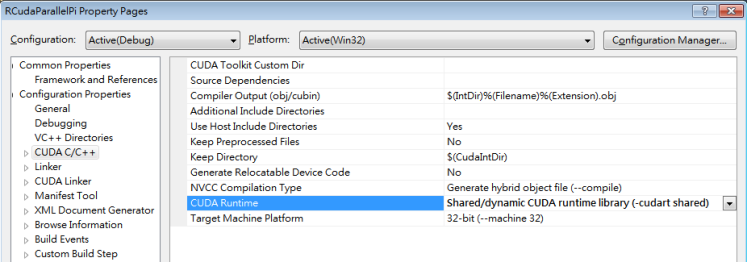
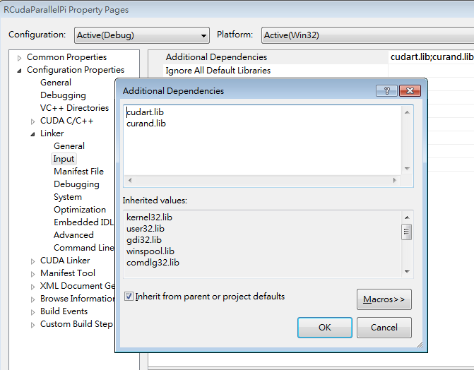
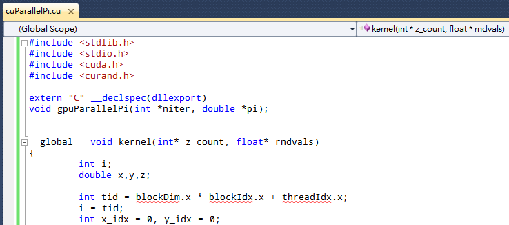
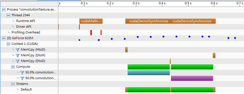
Apart from the traditional methods, modern advances in computing paradigms made possible neural network coupled with specialized hardware, for example GPU, for solving these problem in a manner much more efficiently, especially on huge volume of data. The Python library Theano is a complex library supporting and enriching these calculations through optimization and symbolic expression evaluation. It also features compiler capabilities for CUDA and integrates Computer Algebra System into Python.

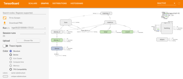
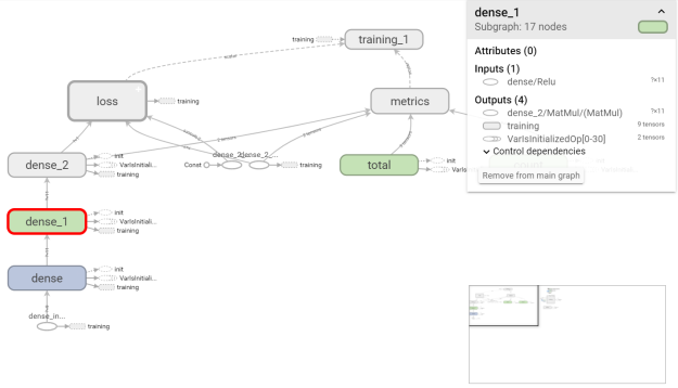
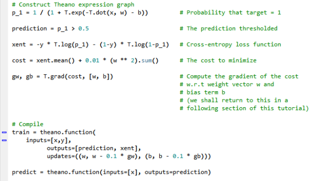
One of the examples come with the Theano documentation depicted the application of logistic regression to showcase various Theano features. It first initializes a random set of data as the sample input and outcome using numpy.random. And then the regression model is created by defining expressions required for the logistic model, including the logistic function and likelihood function. Lastly by using the theano.function method, the symbolic expression graph coded for the regression model is finally compiled into callable objects for the training of neural network and subsequent prediction application.

theanologistic5(theano1)

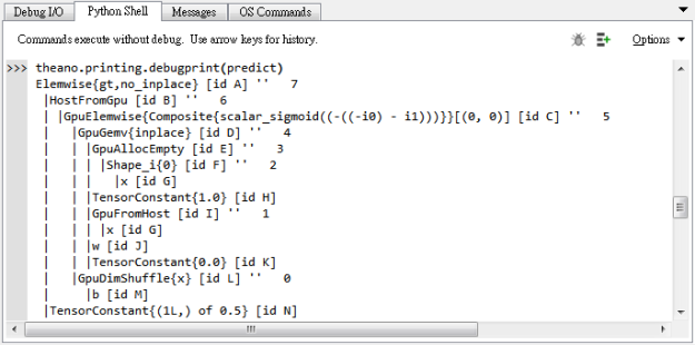
A nice feature from Theano is the pretty printing of the expression model in a tree like text format. This is such a feel-like-home reminiscence of my days reading SQL query plans for tuning database queries.

theanologistic5(theano2).PNG


Implementing parallel GPU function in CUDA for R

There are existing R packages for CUDA. But if there is a need to customize your own parallel code on NVIDIA GPU to be called from R, it is possible to do so with the CUDA Toolkit. This post demonstrates a sample function to approximate the value of Pi using Monte Carlo method which is accelerated by GPU. The sample is built using Visual Studio 2010 but the Toolkit is supported on linux platforms as well. It is assumed that the Visual Studio is integrated with the CUDA Toolkit.

The first thing to do is to create a New Project using the Win32 Console Application template, and specify DLL with Empty project option.

RCuda1
RCuda2

And then, some standard project environment customization including:

CUDA Build Customization:
RCuda3

CUDA Runtime, select Shared/dynamic CUDA runtime library:
RCuda5

Project Dependencies setting. Since the CUDA code in this example utilize curand for Monte Carlo, the corresponding library must be included or else the linking will fail.
RCuda4

Finally the time to code. Only a cu file is needed which resembles the standard directives. It is important to include the extern declaration as below for R to call.
RCuda6

After a successful compile, the DLL will be created with the CUDA code. This DLL will be registered in R for calling.
RCuda7RCuda8

Finally, start R and issue the dyn.load command to load the DLL into the running environment. Shown below is a “wrapper” R function to make calling the CUDA code easier. Notice at the heart of this wrapper is the .C function.
RCuda9

Last but not least, the CUDA Toolkit comes with a visual profiler which is capable to be launched for profiling the performance of the NVIDIA GPU. It can be launched from the GUI, or using a command line like the example below. It should be noted that the command line profiler must be started before R or it might not be able to profile properly.RCuda11

The GUI profiler is equipped with a nice interface to show performance statistics.RCuda10