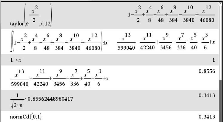
Logistic Regression – from Nspire to R to Theano

Logistic regression is a very powerful tool for classification and prediction. It works very well with linearly separable problem. This installment will attempt to recap on its practical implementation, from traditional perspective by maximum likelihood, to more machine learning approach by neural network, as well as from handheld calculator to GPU cores.

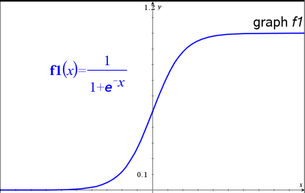
The heart of the logistic regression model is the logistic function. It takes in any real value and return value in the range from 0 to 1. This is ideal for binary classifier system. The following is a graph of this function.

TI Nspire

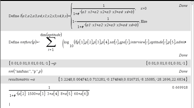
In the TI Nspire calculator, logistic regression is provided as a built-in function but is limited to single variable. For multi-valued problems, custom programming is required to apply optimization techniques to determine the coefficients of the regression model. One such application as shown below is the Nelder-Mead method in TI Nspire calculator.

Suppose in a data set from university admission records, there are four attributes (independent variables: SAT score, GPA, Interview score, Aptitude score) and one outcome (“Admission“) as the dependent variable.

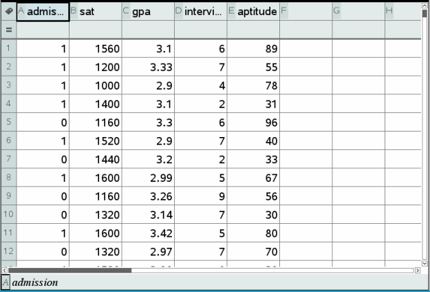
Through the use of a Nelder-Mead program, the logistic function is first defined as l. It takes all regression coefficients (a1, a2, a3, a4, b), dependent variable (s), independent variables (x1, x2, x3, x4), and then simply return the logistic probability. Next, the function to optimize in the Nelder-Mead program is defined as nmfunc. This is the likelihood function on the logistic function. Since Nelder-Mead is a minimization algorithm the negative of this function is taken. On completion of the program run, the regression coefficients in the result matrix are available for prediction, as in the following case of a sample data with [GPA=1500, SAT=3, Interview=8, Aptitude=60].

R

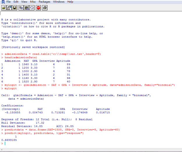
In R, as a sophisticated statistical package, the calculation is much simpler. Consider the sample case above, it is just a few lines of commands to invoke its built-in logistic model.

Theano

Apart from the traditional methods, modern advances in computing paradigms made possible neural network coupled with specialized hardware, for example GPU, for solving these problem in a manner much more efficiently, especially on huge volume of data. The Python library Theano is a complex library supporting and enriching these calculations through optimization and symbolic expression evaluation. It also features compiler capabilities for CUDA and integrates Computer Algebra System into Python.

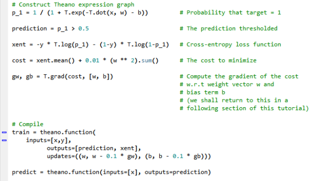
One of the examples come with the Theano documentation depicted the application of logistic regression to showcase various Theano features. It first initializes a random set of data as the sample input and outcome using numpy.random. And then the regression model is created by defining expressions required for the logistic model, including the logistic function and likelihood function. Lastly by using the theano.function method, the symbolic expression graph coded for the regression model is finally compiled into callable objects for the training of neural network and subsequent prediction application.

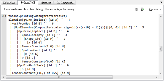
A nice feature from Theano is the pretty printing of the expression model in a tree like text format. This is such a feel-like-home reminiscence of my days reading SQL query plans for tuning database queries.

 

Extracting Black-Scholes implied volatility in Nspire

The Black-Scholes model is an important pricing model for options. In its formula for European call option, the following parameters are required to create a function in the TI Nspire CX:

• s – spot price
• k – strike price
• r – annual risk free interest rate
• q – dividend yield
• t – time to maturity
• v – volatility

Now that the standard Black-Scholes formula is ready, a common method to derive the implied volatility numerically is to determine a value such that the squared loss function between observed price and calculated Black-Scholes price is zero. To derive this volatility, root finding method like the Newton-Raphson method can easily be implemented with advanced calculators like the TI Nspire. In fact, there is no need to code this feature by utilizing the built-in zeros() function of the CX CAS. This function solve for the selected variable from the input expression so that the result is zero, which is exactly what is needed in this case. The function implied_vola() below is coded to do the squared loss function, which is then passed into the CAS built-in zeros() function. Notice a warning of “Questionable accuracy” is reported for the zeros() function.

Doing the Newton-Raphson method is simple enough with the Nspire Program Editor. The program below bs_call_vnewtrap() takes a list of Black-Scholes parameters (including the s,k,r,q,t,v), an initial guess value of implied volatility, and the call price of the standard Black-Scholes formula. The last parameter is a precision control (value of zero default to a pre-set value). The last two attempts calling this function shown below depicts the effect of the precision control in this custom root-finding program.

Approximating normal distribution density function using Taylor series on TI Nspire CX CAS

On the TI Nspire CX CAS, the Taylor series is available as Calculus Series function taylor(). The following is an application of it to approximate the cumulative standard normal distribution. Using order of 12 in the Taylor function below.

How long it takes?

3 minutes on a handheld
3 seconds on an i5